|
Fritz Jooste Administrator Posts: 81
3/11/2020
|
Fritz JoosteAdministrator Posts: 81
To help clients getting started with modelling, we have provided a Default DMS file that can be used as a starting point for modelling.
In the Default DMS, we have assumed what we believe to be a robust modelling approach in which each increment is dependent on a primary and secondary parameter. A key aspect of this model is that it will first use Min-Max Normalization to normalize predictor variables to a value between 0 and 1.
In our default model, we avoid the typical prediction equations used in HDM models. The reason for this is that the HDM models involve exponential terms that can be quite difficult to calibrate for an entire range of expected values. Our default models use a normalized approach that we believe is stable and quite easy to calibrate so that not only the central tendency of predicted increments is accurate, but also, the shape of the predicted distribution is correct (getting the shape of the predicted distribution correct with the exponential regression equations used in HDM can be quite difficult, as explained in this conference paper).
You can control the minimum and maximum values of this normalization, which provides your first level of control over calibration (example provided below).
Once the two predictor variables are normalized, we use the following equation form to predict the Normalized value for the Increment (you can change this to any other equation you like, including ones that rely on more than two predictors):

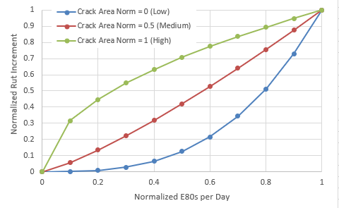
In the above example, the Normalized Rut Increment is determined by (a) the Normalized E80s per Day and (b) the Normalized Crack Area. For both of these parameters, zero indicates low E80s or Crack area and 1 indicates E80 or Crack Area at the maximum expected value. In the DMS, a second calibration factor is provided to control the shape/inflection of the above curves.
Once the model has predicted the normalized increment (value between 0 and 1), an equation is provided to de-Normalize the increment. You again have control over this equation so that you can determine for your network the mapping for de-Normalization. This provides a third potential means of calibrating your model.
Finally, the de-normalized increment can be multiplied by an overall calibration factor K0. Thus, in essence, this model provides 4 levels of calibration. The use of Min-Max Normalization ensures that your model always predicts within a realistic range and numerical errors are unlikely to occur.
As an example, let us say on our network, the observed E80s per day range from 123 to 2345 E80s per day. Then we may choose Min and Max values of 100 and 2500 for the Min-Max Normalization mapping for E80. Thus a value of 2300 (very high on our example network), will get a normalized value close to 1. Conversely, a value of 150 will get a normalized value close to zero.
Looking at the above figure, you can see how these normalized values for E80, together with similarly normalized values for Crack Area, are used to determine a normalized value for Rut increment. For example, for a normalized E80 of 0.4 (roughly middle of range of expected E80 values), and for a normalized crack area of 0.5, the normalized rut increment is 0.3.
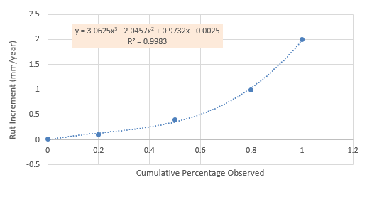
We can now de-normalize this value of 0.3 to get an actual Rut increment. In the default model, we assumed that the following de-normalization relationship applies (you can change this, as explained below):

So from this example, we assumed the normalized rut increment is representative of the Cumulative Percentage Observed. We can now use the above relationship to de-normalize the rut depth. Thus our normalized value of 0.3 will become approximately 0.2 mm/year. You will note in the default DMS we have placed limits to ensure that normalized values always stay in the 0 to 1 range. This ensures stability in the de-normalization process which involves a third order polynomial.
When refining the mapping to de-normalize your increments, you have yet another way to quickly and intuitively calibrate your model. For example, in the figure above you can see that the predicted Rut increments will always be in the range 0 to 2 mm per year, with a median (at the 0.5 x-axis value) of around 0.4 mm per year.
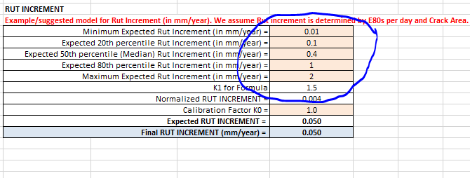
Let us say on your network you have an observed rut range of 0 to 3 mm per year, with a median of 0.5 mm per year. Then you can simply add these values in the areas provided for it as shown below (showing examples from the "Increments" sheet of the Default DMS):

Once you have updated these values, the trend line in the de-normalization curve (graph above) will automatically update. Important! You need to extract the coefficients from the updated trend line equation and enter them in the de-normalization model. You should be able to see where you need to do this, but if you need assistance, feel free to contact Lonrix.
|